SQL Saturday Redmond - Machine Learning for Mere Mortals

10 April 2013

I am privileged to say that I have been chosen to give a presentation at SQL Saturday 212, in Redmond WA, on May 18, 2013.

The topic? Machine Learning for Mere Mortals.

This will be a gentle introduction to the world of machine learning. I will be covering topics including supervised vs. unsupervised learning, clustering, decision trees, association rules, and learning at scale. I shall also provide examples and demos of real-world machine learning applications.

Finally, I’ll provide resources to help people get started.

I hope to see you there!

Buying A Cheap Car Using Data

30 March 2013

December 30th, 2012. 6:00 AM

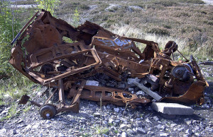
My sister called from her trusted car repair shop. Her car needed a new transmission and fuel pump. She had a ‘95 Ford Escort; major problems like that meant her car was toast. It had been troublesome for months, and was now truly dead.

The car’s demise had left my sister, her husband, and their 2 year old daughter without transport. Worse, they had a 20+ mile commute to work, didn’t have time off, and would be fired if they couldn’t get to work at a moment’s notice.

I had less than 72 hours to find a replacement car. I spoke with my sister about what features she cared about.

• Space for a child seat and groceries
• Reliable
• Purchase price is under $5,000
• Low operating cost

“Operating cost” was the cost to run the car each year: repairs, insurance, and gas.

The goal became a reliable, fuel-efficient car. For under $5,000.

7:00 AM

I had done research into how to buy a car using data. An hour of sleuthing on Craigslist and AutoTrader revealed that vehicles this cheap are 9+ years old and have 100K+ miles on them. Many seemed of dubious reliability.

Unfortunately there was no way to know the reliability of a car from its description. That suggested there were both ripoffs and deals in the listings. This was an information asymmetry problem. The seller had close to perfect knowledge and the buyer had very little.

8:00AM

Internet sleuthing led me to FleetBusiness, which reported how long different brands last before they die (are junked). I also found TrueDelta, which had reports from car owners about what car repairs, mileage and cost.

I quickly graphed the FleetBusinss data showing scrap rates of different brands of car. I conflated age with mileage/wear; I couldn’t avoid the confound given the time.

The car brand that died off quickest was Suzuki. The brands that died off slowest were Toyota, Honda and Subaru. The die-off rate was not a straight line…it was an S-shape, like the continuous normal distribution. Looking at the scrap rate per year, I saw a roughly normal distribution:

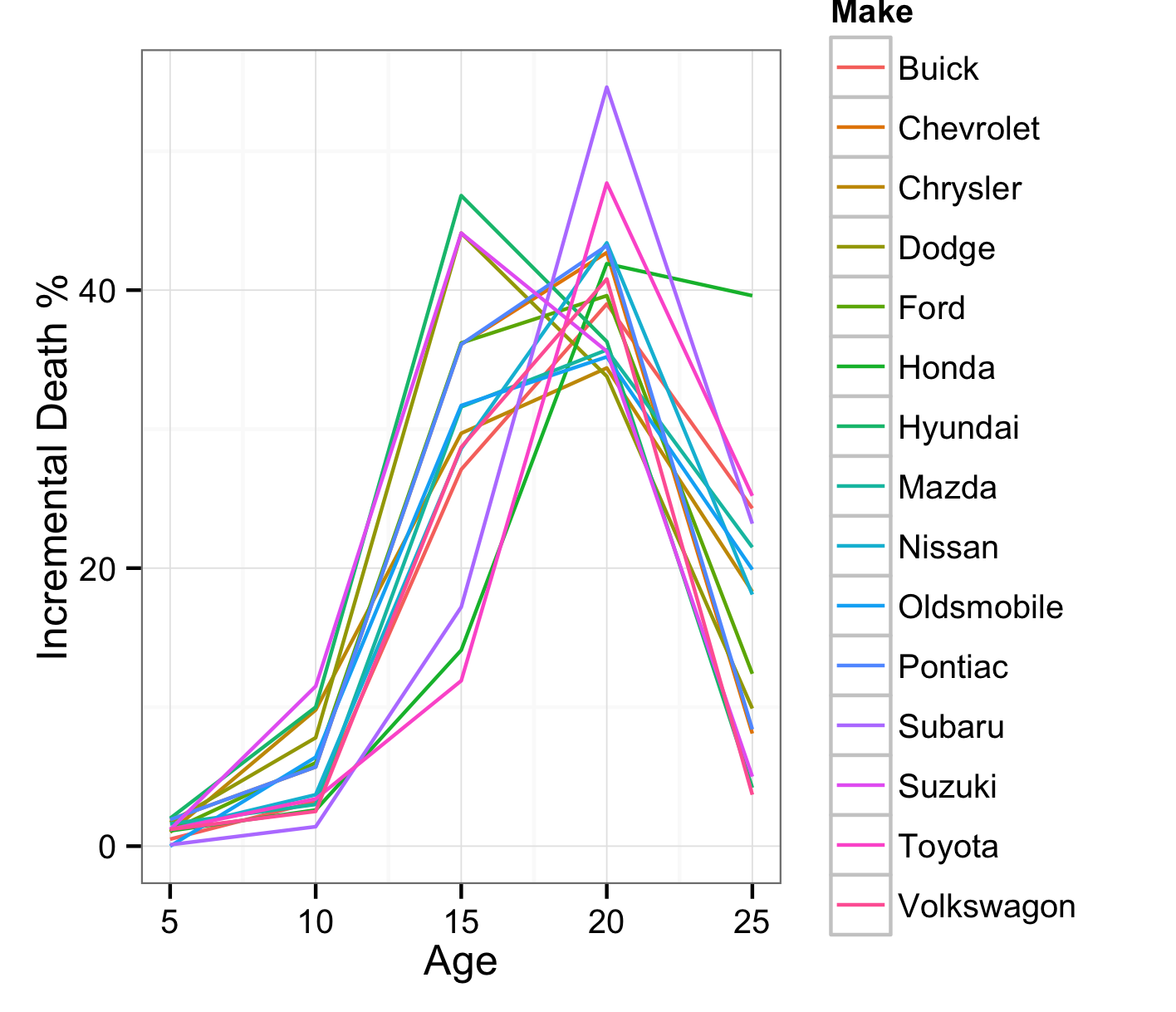
I also saw that cars died off en masse at 10-20 years old. The cars I was looking at were the worst possible age. The odds were good the car I purchased would die within the next 5-10 years.

I didn’t care about total car death rates; I cared about how long a car would last if I purchased it at a certain age. The cars I was looking at purchasing were 10-13 years old. Any cars that died before that age were not for sale so I could exclude that percentage.

I subtracted the 10-year death rate from each year’s death rate:

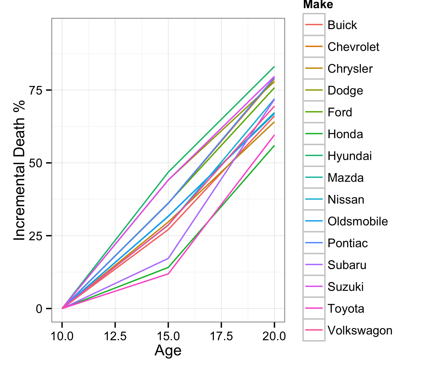
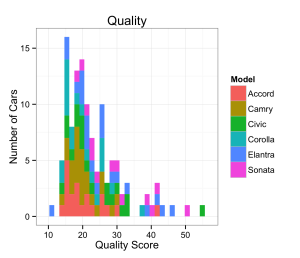
The most reliable brands to buy at 10 years’ age were Honda and Toyota followed by Chrysler. I picked 6 reliable models:

• Toyota Corolla
• Honda Fit
• Honda Civic
• Toyota Camry
• Hyundai Sonata
• Hyundai Elantra

I had added 2 Hyundai models, the Elantra and Sonata, because I had heard their later-generation models were well built. This was not data-driven and stupid.

9:30AM

I started gathering data from car listings (for-sale ads). My goal was to have enough listings that I could be confident there were a few good deals. I excluded any listing that didn’t have the car’s year, model, mileage, and price listed. After a few hours I had 117 cars listed.

12:00PM

The biggest cost of owning a car is depreciation: the difference between your purchase price and what you sell it for. The best way to reduce that cost is to buy it as cheaply as possible and keep it running for as long as possible.

</a>

I didn’t really care about how many miles a car had or its age. I wanted a car with as many miles remaining as possible. I needed to find out how long each car model would last. If you buy a car with 125K miles on it, there’s a big difference between a car that will last 200K miles and 150K miles. The 200K car will go 300% as far.

A car’s mileage is more important its age. For the same price, which is a better car?

• 4 years old and 200K miles
• 8 years old and 100K miles

The 8-year-old car is a better choice. I guessed that mileage was roughly 5X more important than age. I knew maintenance costs would increase exponentially as mileage and age increased. I puzzled out an equation to compute a ‘reliability score’ for each car.

Score = fnNormalize ( Age ^ 1.2 ) * 20% + fnNormalize ( Mileage ^ 1.4 ) * 80%

The ratio of this score to the price is the ‘value score’. Cars with higher value scores were better deals:

I saw that, roughly, better-quality cars were more expensive. However, it was a general trend and not a clearly linear relationship. There were ripoffs (in the upper left, with smaller points) and great potential deals (in the lower right, with larger points).

Now I had a shopping list: the 5 cars with the highest value scores. I quickly called the top 3 car owners to ask if the cars were still on sale and available for a test drive. After a nap.

2:00 PM

I met with my sister and family for lunch. Afterwards we went to see the #3 car at a nearby dealership. We went prepared with a to-check list.

The test drive was illuminating: the car was junk. The brakes barely worked, the fan belt made a loud whistling sound, the window seals were crumbling and the lowest gear didn’t work…in an automatic. We left in a hurry.

4:00 PM

The owner of the first car on my list called back, saying that the car had just sold. Darn.

The owner of the car #2 called: the car was still for sale! I guessed the car would sell quickly and arranged for a test drive that evening.

I called car owner #4 on my list, leaving another message. I wasn’t confident car #2 would work out so I wanted to keep looking. After another break.

7:00 PM

I wasn’t hopeful of finding a good car after that first test drive, and was surprised when this car handled well. The engine, brakes, steering, and lights all worked perfectly. A roller-coaster route through West Seattle found no issues.

The owner had copies of their maintenance logs for 3 years and seemed trustworthy. We quickly made plans for my trusted mechanic to look over the car the next day. I would buy the car if it passed a mechanical inspection.

9:00 PM

The car and seller were legitimate. A check of the vehicle’s VIN number against both AutoCheck and the NICB Stolen Car Database found nothing amiss: no thefts or accidents.

A Google search of the seller’s name, email address and phone number confirmed her identity. Her name matched her online photo and she had enough of an Internet presence to be legit. This felt vaguely creepy, but also prudent given the money involved.

December 31st, 2012, 9:00 AM

I arranged for an afternoon test-drive with car #5. I explained that I had a better lead that may not pan out; the seller was very understanding.

11:00 AM

The mechanic confirmed car #2 was in good working condition except the it burned some oil when accelerating. Some hasty Internet searches suggested this was not unusual for old Toyota Corollas and didn’t mean the engine was toast. Success!

1:00PM

My sister and her family arrived at the auto repair shop, we signed all the paperwork, paid the seller, and went our separate ways.

Time to Complete: 31 Hours

Epilogue

• I have put all of my code, data and analysis on GitHub.
• Work quickly. Good deals sell fast, in a day or two. It helps to look at several cars at once because your best choices won’t last long.
• Hundreds of cars in Seattle were listed on Craigslist and AutoTrader each day. That’s good and bad: you could find new deals every day, but had to look continuously to stay informed.
• All of the private sellers I spoke with were very polite, even friendly. It helped when I explained my sister’s situation. People are sympathetic.
• Craigslist posts were often incomplete (no price, mileage, or just spam). The formatting was so bad that it was faster to collect the data by hand than write a script to do it.
• The dealer car we tried was far in worse condition and more expensive than the private seller. A recent NADA report shows that used-car dealerships profit margins of 12% for used cars. That means a $5,000 car at a dealership would cost $4465 on by a private seller.
• This is a common situation. 38.8 million US households make less than $30,000 per year, and usually need a car for work. They have little savings and lots of debt. The average car lasts ~11 years. If 75% of poor households have at least one car, this situation occurs 2.6 million times a year. If the average used car costs between $3000 and $8000, that’s an industry of $8 to $20 billion per year.
• If we assume 1/2 of the cars are purchased through dealers at a 12% markup, that’s a $418 million to $1.14 billion markup for little customer value.
• This is not a problem that’s quickly automated. The quality of a car is not easily determined by the online information. You have to take it to a mechanic.
• A group of car-repair shops in the city could make a killing. They could provide an independent, trusted ‘report card’ on each car for sale. Put that online, charge for it, and voila, a business.
• There is a lot of hidden data that would make decisions easier. If the goal is to drive a car until it dies, we need to know how many other cars of that same make, model & year lasted before they died. That information exists in the databases of various state Departments of Licensing.
• Price negotiations change all of this math.
• I don’t know anything about auto finance for cars this cheap. I suspect there isn’t any, or it’s a bad deal. Having savings is far, far easier.
• It helps to have a car when doing car searches to get around. ZipCar, Car2Go, or borrowing a car from a friend/relative are good options.
• There are many sites that purport to help with car buying but do not provide useful data. Examples include TrueCar and Hedges & Company. They often focus solely on new cars.
• There are also governmental sites such as the US DOT but they don’t provide enough data either. There’s an emphasis on function-specific reports instead of exposing raw data.
• I suspect the cheapest way to own a car is to buy something a little newer, (say, 5-6 years old) because it’s only marginally more expensive but miles left on the car are likely to be far higher.