Find Good Schools Using Data - Part Three

11 February 2013

Schools produce data. Thus far we have looked at school quality, and its relationship to house prices. What else affects the quality of school? School size? Parents’ education? Teacher salaries? Gender ratios? Teacher ratings?

Can we use this knowledge to make better decisions?

Brains > Algorithms

First, look at data. A common challenge in data analysis is knowing the appropriate methods to use. There are thousands of statistical and machine learning algorithms, and none of them are appropriate for all situations. Let’s see some density plots of different variables:

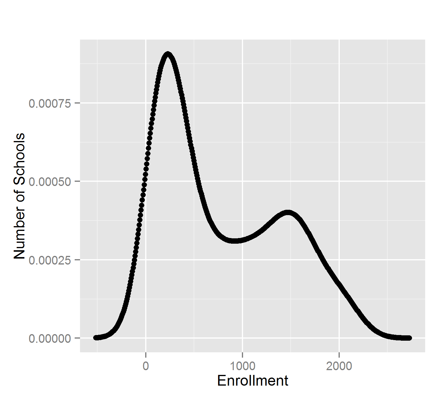
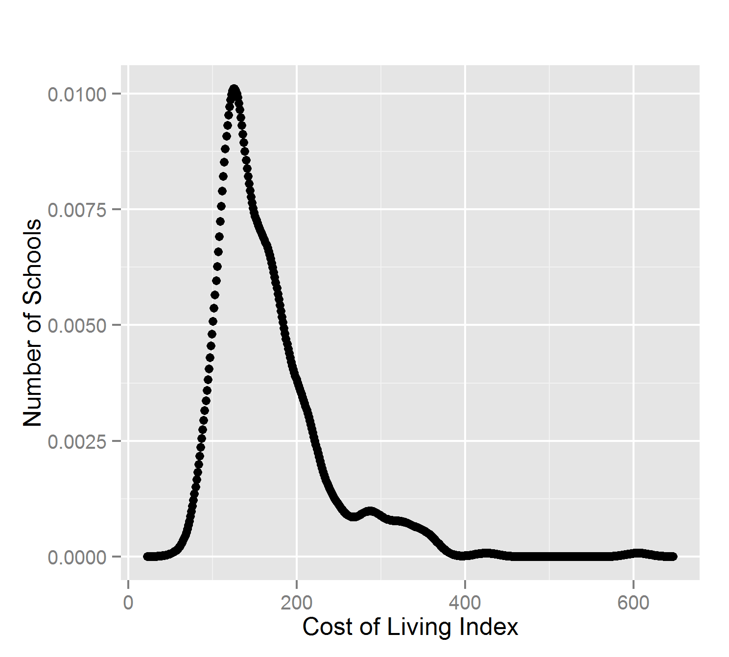
What do we see? High schools appear to come in two different size ranges. The cost of living has a positive skew. School budgets are relatively similar.

None of these attributes follow a ‘normal’ (Gaussian) distribution of values. The most common statistical methods are therefore inappropriate: mean, standard deviation, and Pearson’s correlation.

Let’s see which variables correlate well with High Achiever %. We can’t use Pearson’s correlation here, so we’ll use Spearman’s Rho instead.

Some variables have a strong correlation, such as parents’ education levels. Others don’t, such as the age of the school neighborhood.

We must remember that correlation does not imply causation. However, the lack of a correlation does imply a lack of causation. If two variables are not correlated then there a causal relationship is unlikely, if not impossible.

Peekaboo, How Good Are You?

Let’s use a combination of factors to predict the quality of school. We’ll use a machine learning algorithm, Random Forests, an ensemble method of decision trees with good behavior for this class of problem.

A few lines of code produce a model to predict school quality. Let’s see how closely the predicted (green) values compare against the actual (red) values:

Good, but not perfect. It is impressive that we can predict school quality using only demographic and budget data. After all, we don’t have any information about teacher skill, different teaching techniques, or the students themselves.

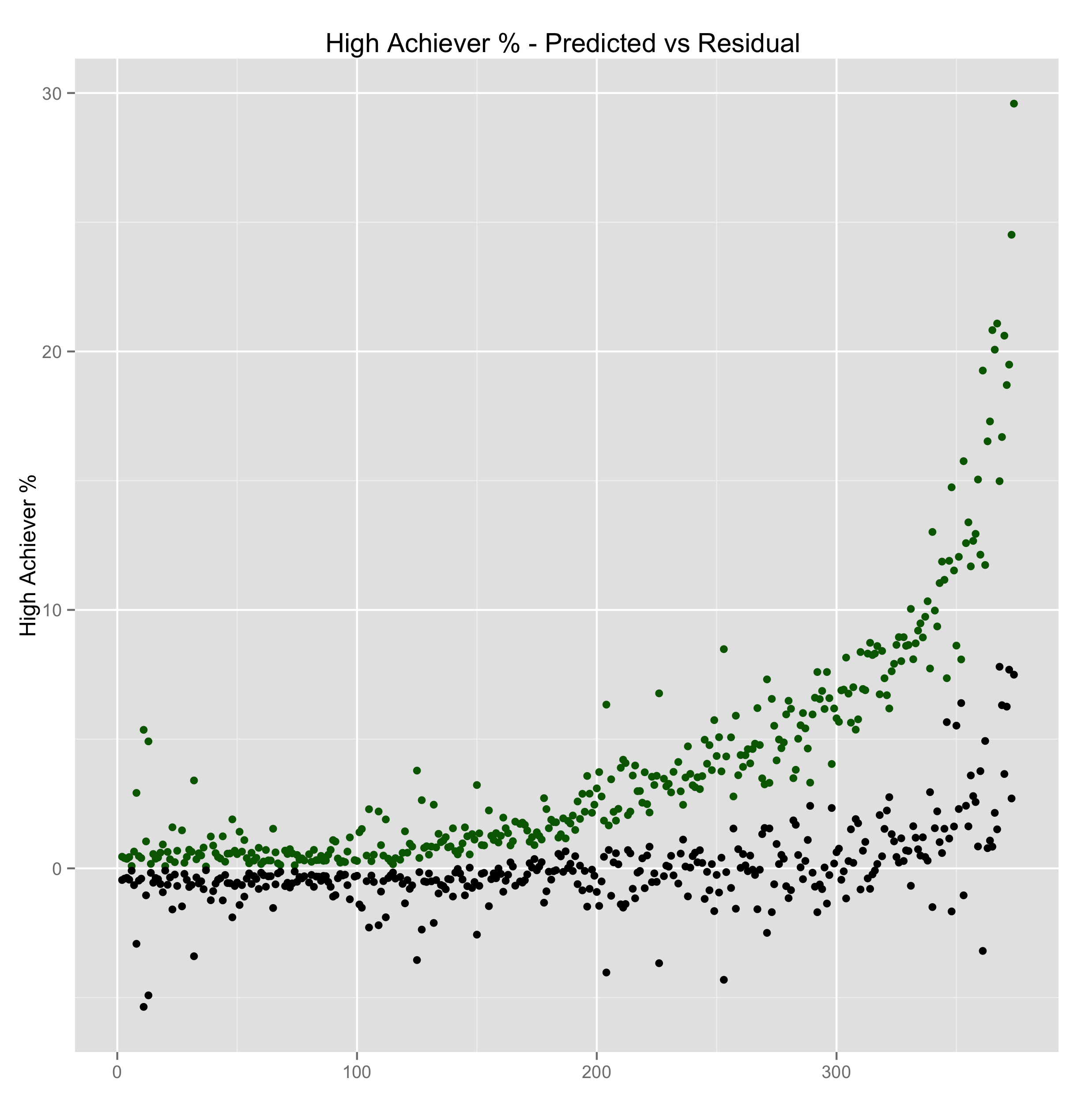
Let’s plot the residual (actual - predicted), values, in black, against the predicted numbers, in green. The residual numbers contain variation that is not explained by demographics or budgets. They suggest that unobserved variables are involved, like teacher skill or student aptitude.

Let Data Be Your Guide

Analysis thus far suggests school quality is influenced by demographics and budgets. These are factors a school cannot control.

Let’s use that to our advantage. Groups of schools with similar demographics will still have different levels of quality. They can learn from each other, since schools in similar situations have done well.

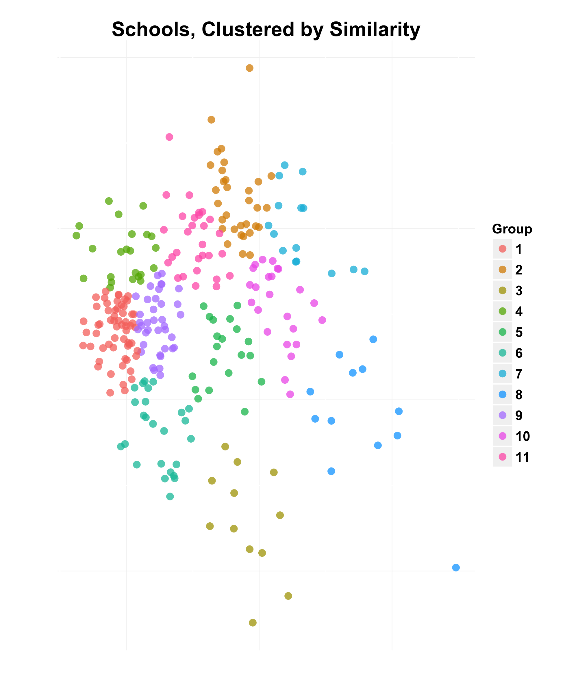
Let’s group schools together using another algorithm, k-means. It belongs to a set of machine learning techniques for clustering.

The k-means algorithm has a limitation: it groups together objects by first computing the Euclidean distance between each. Euclidean distance treats each variable as equally important, which is not true for this example. We will compensate for this by ‘weighting’ each variable according to its importance, which the random forest algorithm has already calculated.

We can then assign a group to each school, clustering together similar schools into the same group.

Let’s look at the High Achiever % of each group.

As we can see, each group has some spread of values. This is encouraging, because these schools could learn from each other. High schools of similar size, with similar parental situations and similar demographics are likely to have relevant advice for each other.

Share and Share Alike

This leads me to a triumvirate of conclusions:

Schools/Educators: You aren’t alone. There are many other schools just like yours, doing better and worse. Ask for help in finding them. Then learn from them, and teach in turn. Identify best and worst practices specific to your situation. Spread that information around. The more schools that participate, the more everyone benefits.

Parents: Teachers and principals have limits to their ability to educate children, and it depends on many things. You have a much more profound impact on your children’s education than their teachers do. You can’t dodge that responsibility, so don’t try. And for goodness sake, be careful about what data you pay attention to. Good test and SAT scores don’t predict whether your child will be happy or successful in 10 years.

Analysts/Data Scientists: Like all professionals, we have a choice of what to do with our talent. Each of us has access to huge amounts of data. We can use our skill and energy to make the world a better place. I encourage everyone to try.

Compressing Tabular Data

11 January 2013

I have a bandwidth problem. I am a software developer who builds services using ‘the cloud’. I have to copy large amounts of data between datacenters, like those run by Amazon Web Services or Microsoft’s Azure. Such WAN copies are predominantly slow and pricey. Much of the the data is tabular (stored as rows and columns). I use .csv files a lot. I need bigger tubes.

A solution is to compress the files. CSV files compress somewhat well. CPU capacity is cheap and abundant, especially compared to network bandwidth. Like all software developers, my solutions must optimize for cost and speed.

There is still a problem for large data sets. Even with 90% compression (1 TiB -> 10 GiB), data transfer takes time. There is a better way.

It’s All About the Algorithms

The key is to understand compression algorithms. They analyze one file at a time, in sequential order, looking at blocks of data. The more alike the data blocks, the better the compression.

Csv files compress inefficiently, because a csv file is stored row by row. The data across a row can be very different (for example: numbers, strings, dates, decimals). The data down an entire column is likely to be very similar (for example: all numbers or all dates).

A better way to compress tabular data is column by column instead of row by row. This is already part of large-scale data tools like Vertica, SQL Server’s Columnstore indexes, and Cassandra’s secondary indexes.

A simple way to turn a CSV file into a column-oriented (columnar) format is to save each column to a separate file. To load the data back in, read a single line from each file (column), and ‘stitch’ the data back together into a row.

Show Me the Numbers

All algorithms should be tested. The ‘data_per_formatted’ data from a Kaggle competition is a good test set. The csv file is 7.69 GiB uncompressed. The columnar set of files for this data is the same size.

A simple Powershell script ran both csv and columnar data sets through 20 different compression tests, using 7Zip as the compression tool. Each test recorded the time to compress and the resulting file size. The tests themselves were run on a desktop.

The columnar data compresses more efficiently than the csv data. It can also be faster.

As we can see, the best csv test reduced the data to 581 MiB. The best columnar test reduced the data to 402 MiB, which is a 31% improvement. Equally important, columnar data compresses better than csv data no matter which compression algorithm you use.

Time to Copy

The goal is to reduce the time to copy data from one place to another, including the time to compress and decompress the data.

Using compression is almost always a good choice. Its time advantage decreases only when the network speed approaches the speed of compression itself.

Compression is most appropriate for data in a certain size range, between 1 GiB and 20 TiB. Smaller data sets don’t take very long to copy. Larger data sets larger are best copied using the massively scalable bandwidth of FedEx.

These problems aren’t going away. The continuing rise of distributed system architectures, cloud computing, larger data volumes guarantees, and IT budgetary pressure guarantee that. Dramatic improvements in speed and cost can be achieved by applying existing tools in unexpected ways.